
Modeling Marketing Drivers Using a Regression Model
Introduction
Oftentimes in Marketing Analytics, we want to understand how well the company’s Media campaigns contributes to sales.
This work helps inform the Marketing department what creatives, Marketing channels, and tactics are working. One of the most effective ways to understand which drivers are contributing to sales is to use a multiple linear regression model to model sales on a time series.
Forecasting vs Driver Modeling
Building models on a time series involves models that take the past data of the metric, in this case sales, and forecast what the sales would be in the future.
Here are the models that are often used:
- Moving Average
- Exponential Smoothing
- Seasonal decomposition
- Auto Regressive Models such as ARIMA and SARIMA
- Facebook Prophet
There are more advanced models that use neutral networks such as Neural NETwork AutoRegression and LSTM models (Long-Short Term Memories) as well.
All of these popular models focus on predicting our metric (sales, transactions, units, etc..) based on past observations of our metric; these models focus on predicting future observations.
However in the Marketing world, Marketers often want to understand which campaigns, tactics, and media channels have the most effect on sales throughout the calendar year. In this case, building a forecasting model does not help marketers understand which campaigns have a significant contribution to sales. For this case, we would need to build a Driver model that seeks to understand which campaigns and channels significantly drive sales.
There are two models I’ve come across that can do this:
- Multiple Linear Regression (MLR)
- Bayesian Hierarchical Modeling
We’re going to focus on building a MLR model to understand different Marketing drivers.
Note: The following sections assume you have a basic understanding of how to build a MLR model and know how to read the statistical outputs of the MLR model. If you don’t know how to build a basic MLR model, you should stop here and learn how to build an MLR model first before continuing.
Regressions with Seasonality
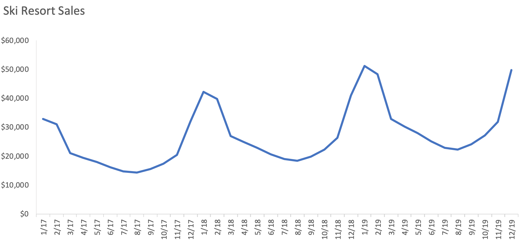
When modeling a time series, we often have seasonalities that we need to account for. Most businesses have sales that rise and fall depending on the day or month of the year. For example, a ski resort’s sales will be highest during the winter months and lowest during the summer months.
However, when we create a regression, we usually use linear terms that output a straight line. True, we can use polynomial terms to help model the peaks and valleys, but seasonality is not dependent on any one coefficient and therefore using polynomial terms is not a viable solution.
Seasonality by definition repeats itself. Notice how these peaks and valleys look similar to a sinusoidal wave. In other words, seasonality is a periodic signal that can be modeled using a Fourier Series.
Fourier Series
Therefore we can model the seasonal part of the time series using a combination of sine and cosine functions within our linear model:
\[f(x) = \alpha_0 + \alpha_1\cos(2\pi T_1) + \beta_1\sin(2\pi T_1) + \gamma_1x_1 + \gamma_2x_2 + ... + \gamma_nx_n\]\(T_n\) = time/frequency for n
Where time is a positive integer, representing the point in time starting at 1 and frequency is a positive integer, representing how many points in time it takes for the period to repeat. For yearly seasonality with monthly data points, frequency would be 12 because the year repeats itself every 12 months.
If we’re modeling data that has multiple seasonalities, we can increase the order of the cosine and sine functions to model additional periodic signals. For example, we may model daily data that has a weekly seasonality (Tuesday sales tend to be higher than the rest of the days in a week) and monthly seasonality (Winter months tend to be higher than the rest of the months in a year).
In this case, we would add an additional \(\alpha_2\cos(2\pi T_2) + \beta_2\sin(2\pi T_2)\) to our regression model with frequency 7.
You can read more about the theory and applications of Fourier Series here.
Application
Let’s go back to the Ski Resort example and assume this scenario. We’ll be using this data here. Feel free to follow along and build the model along with me.
The Marketing department launched 3 new Social media campaigns in 2019 and noticed that sales have grown in 2019 relative to 2018. The Chief Marketing Officer (CMO) would like to know which campaigns worked the best in terms of driving sales in 2019. This would help the CMO decide which campaigns to keep and which campaigns to modify for the 2020 Marketing plan.
We assume we have data for three years starting from January 2017. The data contains the following columns:
- Sales
- Month
- Membership Fees: Monthly fees from Elite Ski Resort members
- Campaign 1: Contains social impressions by advertising agency
- Campaign 2: Contains social impressions given by advertising agency
- Campaign 3: Contains social impressions given by advertising agency
In Marketing, metrics used to track social and media campaigns often are:
- Social Impressions
- GRPs and TRPs
- Click through Rates
- Return on Ad Spend
Assume that our team knows that we should use social impressions for social campaigns because it’s the most reliable metric.
| month | sales | membership_fees | campaign_1 | campaign_2 | campaign_3 |
|---|---|---|---|---|---|
| 1/1/17 | 31206 | 1449 | 0 | 0 | 0 |
| 2/1/17 | 29381 | 701 | 0 | 0 | 0 |
| … | … | … | … | … | … |
| 4/1/19 | 30292 | 800 | 13084 | 16000 | 0 |
| 5/1/19 | 27909 | 698 | 0 | 14998 | 0 |
Feature Additions
Assume that we’ve done our due diligence and checked for multicollinearity across all our features; we should always do this whenever we create a MLR.
Next, we add a new feature (or column): T that contains the time/frequency for each month. Since the seasonal pattern repeats itself every 12 months, frequency is 12.
| T | month |
|---|---|
| 1/12 | 2017-01-01 |
| 2/12 | 2017-02-01 |
| … | … |
| 36/12 | 2019-12-01 |
Next we add in the Cosine and Sine columns to help model out the present seasonality.
| T | \(\cos (2\pi T_n)\) | \(\sin (2\pi T_n)\) |
|---|---|---|
| 1/12 | 0.86603 | 0.5 |
| 2/12 | 0.5 | 0.86603 |
| … | … | … |
| 36/12 | 1 | \(6.4 \times 10^{15}\) |
We then run an MLR model on the following features: membership fees, campaign 1, campaign 2, campaign 3, cosine, and sine with the dependent variable: sales.
Results
Let’s graph the predicted sales of the MLR model against actual sales.
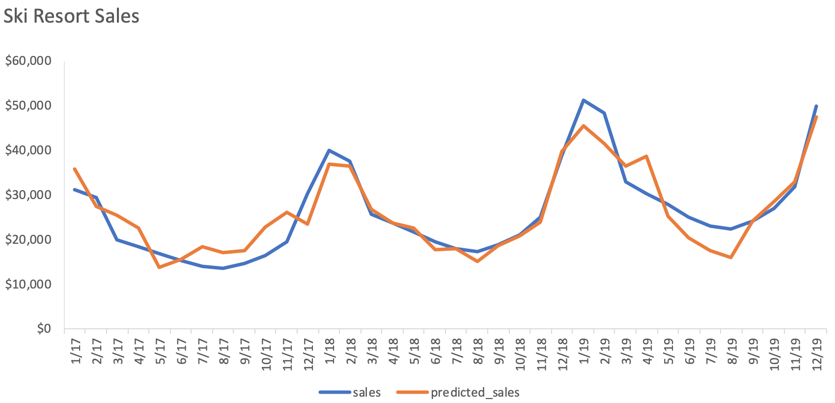
We see here that the model fairly creates a decent job at modeling out the seasonality curves. The Adjusted R-squared turns out to be 0.81.
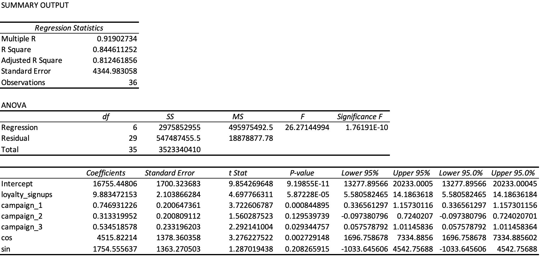
Here is that statistical report from the MLR model along with a graph of the Standardized Residuals.
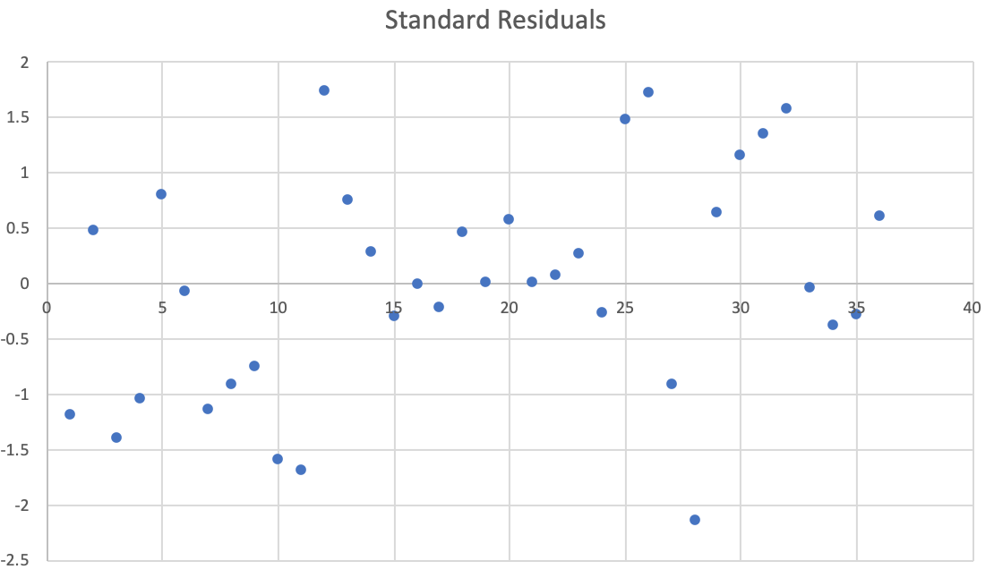
We can see here that the residuals are fairly homoscedastic, which is what we always want when creating a regression model.
Interpretation
For driver models, we can have higher alpha levels because we’re not using these models to make predictions. In this case, we’re willing to accept an alpha level of 15%.
Therefore the coefficients for all three campaigns can be used to help explain sales contributions for our model since their respective P-values are under 15%.
From the coefficients, we know that Campaign 1 (coefficient 0.75) is the most successful, followed by Campaign 3 (coefficient 0.53). If we look at the data, it makes sense because both of these campaigns occurred during the Winter and Fall months while Campaign 2 (coefficient 0.31) occurred during Spring and Summer.
The CMO wants to know sales contributions (instead of coefficients) for the year 2019; this is basically a sales mix among all of our features.
To calculate this, we sum up all of the data for 2019 for all features and multiply each sum by each coefficient to get the total sales for each feature for 2019.
| membership_fees | campaign_1 | campaign_2 | campaign_3 | cos | sin | intercept | |
|---|---|---|---|---|---|---|---|
| Coefficients | 9.88 | 0.75 | 0.31 | 0.53 | 4515.82 | 1754.556 | 16755.44806 |
| 2019 Sales | $ 95,138.30 | $ 38,946.49 | $ 15,798.85 | $ 23,665.81 | $ 0.00 | $ 0.00 | $ 201,065.38 |
| Sales Contribution | 25% | 10% | 4% | 6% | 0% | 0% | 54% |
Next, we calculate the sales mix for each feature. We would report out to the CMO that Campaign 1 contributed 10%, Campaign 2 contributed 6%, and Campaign 3 contributed 4% to overall 2019 sales.
We would then make recommendations to reevaluate Campaign 2 and to invest more money in Campaign 1 and Campaign 3 next year.
Summary
Driver modeling is a useful tool to help Marketer’s evaluate Marketing efficacies. The models help inform Marketers what activities and campaigns significantly drive the business. Rather than using a seasonal decomposition model, we can use a MLR with Fourier terms to model out seasonality on a time series.
More complex models such as Hierarchical Bayesian Models do exist. These models create multiple levels (hierarchies) of data that can uncover robust insights and relationships between multiple Marketing metrics (impressions, GRPs, Return on Ad Spend, etc).
This would require running several simulations to reach posterior distributions, which would be the final coefficients of the Bayesian model. If you want to dive deeper in Bayesian analysis, I recommend this book by John Kruschke, Doing Bayesian Data Analysis: A Tutorial with R, JAGS, and Stan.
Click here to download the final regression work done in Excel.