Understanding the Mechanics of Bayes Theorem
Introduction
Continuing my journey into Bayesian Statistics, I finally developed a firm grasp of the actual mechanics involved in calculating posterior probability distributions. Will Kurt’s book “Bayesian Statistics The Fun Way” did an amazing job explaining Bayes Theorem and how to actually use it to calculate posterior distributions.
This post will focus on applying Bayes Theorem showing you how to actually calculate the posterior distributions using the Beta distribution.
Bayes Theorem
Bayesian statistics is simply an exercise to compare different beliefs we have about the world given some set of observed data.
We already intuitively do this reasoning every day, every hour of our lives. Given some sort of observation in the real world, what happened that produced the observation?
For example, I come home and find my door unlocked. What are the possible beliefs that led to my door being unlocked? Did I forget to lock the door? Did my roommate forget to the lock the door? Did a burgler break into my house?
Each of these beliefs I mentioned will have a certain probability. Knowing myself, there’s a higher chance that I forgot the lock the door vs a burgler breaking into my house given my past behavior and where I live; but just how much more?
Bayesian statistics gives us a way to precisely quantify the strength of our beliefs given our observations.
And if we have many different beliefs, the Bayesian method allows us to precisely assign credible probabilities among all the possible beliefs to help us choose the right beliefs that model the data appropriately.
According to Dr. John K. Kruschken of Indiana University:
All we’re doing is allocating credibility across possibilities.
The Formula
In general, Bayes Theorem is defined as:
\[P(H|D) = \frac{P(H)P(D|H)}{P(D)}\]where H = Hypothesis, D = Data
If you’re not familiar with this notation, P(H) means the probability of H occurring while \(P(H|D)\) means the probability of H occurring given D has occurred.
What this formula means is that given a hypothesis that we have in this world, we can determine how strong our Hypothesis is given an observed set of data.
This formulaic approach gives us a method to quantify our beliefs in a precise and objective way, giving us the ability to compare different beliefs or hypotheses.
There are four components of Bayes Theorem:
\(P(D|H)\) is called the likelihood of the observed data occurring given that H exists. This tells us that given a belief we have, what is the probability of this data occurring?
\(P(H)\) is called the prior probability. The prior probability helps shape the final posterior probability of \(P(H|D)\). This is the source of many controversies in Bayesian analysis because it could lead to many arguments on what is the “right” prior probability to use. We often bring in prior data and observations to help inform the prior probability.
\(P(D)\) is called the evidence. It’s used as a normalization factor to guarantee that the posterior probability will always produce a number between 0 and 1.
All of these components lead us to \(P(H|D)\) that precisely tells how strong our belief is given the observed data.
Beta Distribution
We can explore how to calculate the posterior probability by using the Beta distribution. The Beta distribution is a simple distribution that allows us to analytically calculate the prior and posterior distributions.
The Beta distribution emerges by counting the number of successes out of \(n\) number of events.
For example, we can count the amount of clicks from people opening a marketing email from an email campaign. The Beta distribution takes two parameters: \(\alpha\) and \(\beta\).
\(\alpha\) = number of successful events
\(\beta\) = number of unsuccessful events
where \(n = \alpha + \beta\)
Let’s rewrite Bayes theorem using a different notation to connect Bayes theorem with our Beta distribution model:
\[P(\phi|D) = \frac{P(\phi)P(D|\phi)}{P(D)}\]where \(\phi\) is the set of parameters that represents a model that we believe explains the data \(D\) we see. From here, we can now play with different models as well as model parameters to quantify how well the data can explain our model.
Note: For the last part of this article, I’ll be including the R code I used to generate the following graphs so you can follow along and code everything yourself.
Let’s define a function to help us plot the beta distribution given the parameters, \(\alpha\) and \(\beta\) and R’s dbeta function.
plotbeta <- function(alpha,beta,xs,ylim) {
  plot(xs, dbeta(xs,alpha,beta),type='l',lwd=3,ylim=ylim,
       ylab='density',
       xlab='probability of clicks',
       main=paste('PDF Beta(',alpha,',',beta,')'))
}
Let’s graph the Beta distribution with \(\alpha = 2\) and \(\beta = 3\):
alpha = 2
beta = 3

xs.all <- seq(0,1,by=0.0001)
xs <- seq(0,0.15,by=0.0001)

plotbeta(alpha,beta,xs.all,c(0,2))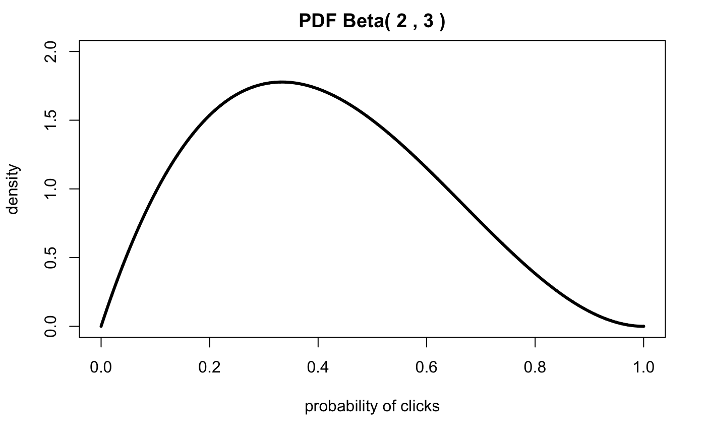
Let’s graph several more Beta distributions with different alpha and beta parameters:
alpha.1 <- 1
beta.1 <- 41

alpha.2 <- 2
beta.2 <- 80

alpha.3 <- 5
beta.3 <- 200

plot(xs, dbeta(xs,alpha.1,beta.1),type='l',lwd=3,
     ylab='density',
     xlab='probability of clicks',
     main='Different Beta Distributions')

lines(xs, dbeta(xs,alpha.2,beta.2),lty=2,col='red',lwd=3)
lines(xs, dbeta(xs,alpha.3,beta.3),lty=4,col='blue',lwd=3)
legend(x='topright',
       legend=c( paste('Beta(',alpha.1,',',beta.1,')'), paste('Beta(',alpha.2,',',beta.2,')') , paste('Beta(',alpha.3,',',beta.3,')')),
       col=c('black','red','blue'),
       lty=c(1,2,3),
       ncol=1 )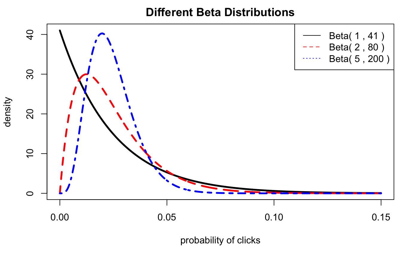
Calculating Posterior Probabilities with the Beta Distribution
Using the Beta distribution, we will now walk through how one would apply Bayes Theorem to calculate our posterior probabilities: \( P(\phi|D)\) by using our prior probability to re-allocate the probabilities we saw from our likelihood.
Assume that we have an email campaign we’re tracking. For the first 5 minutes, 10 emails have been sent out and 3 people have clicked on the link in the email campaign.
Therefore our likelihood is driven by the model parameters:
\(\alpha = 3\)
\(\beta = 7\)
alpha = 3
beta = 7
plotbeta(alpha,beta,xs.all,ylim=c(0,13))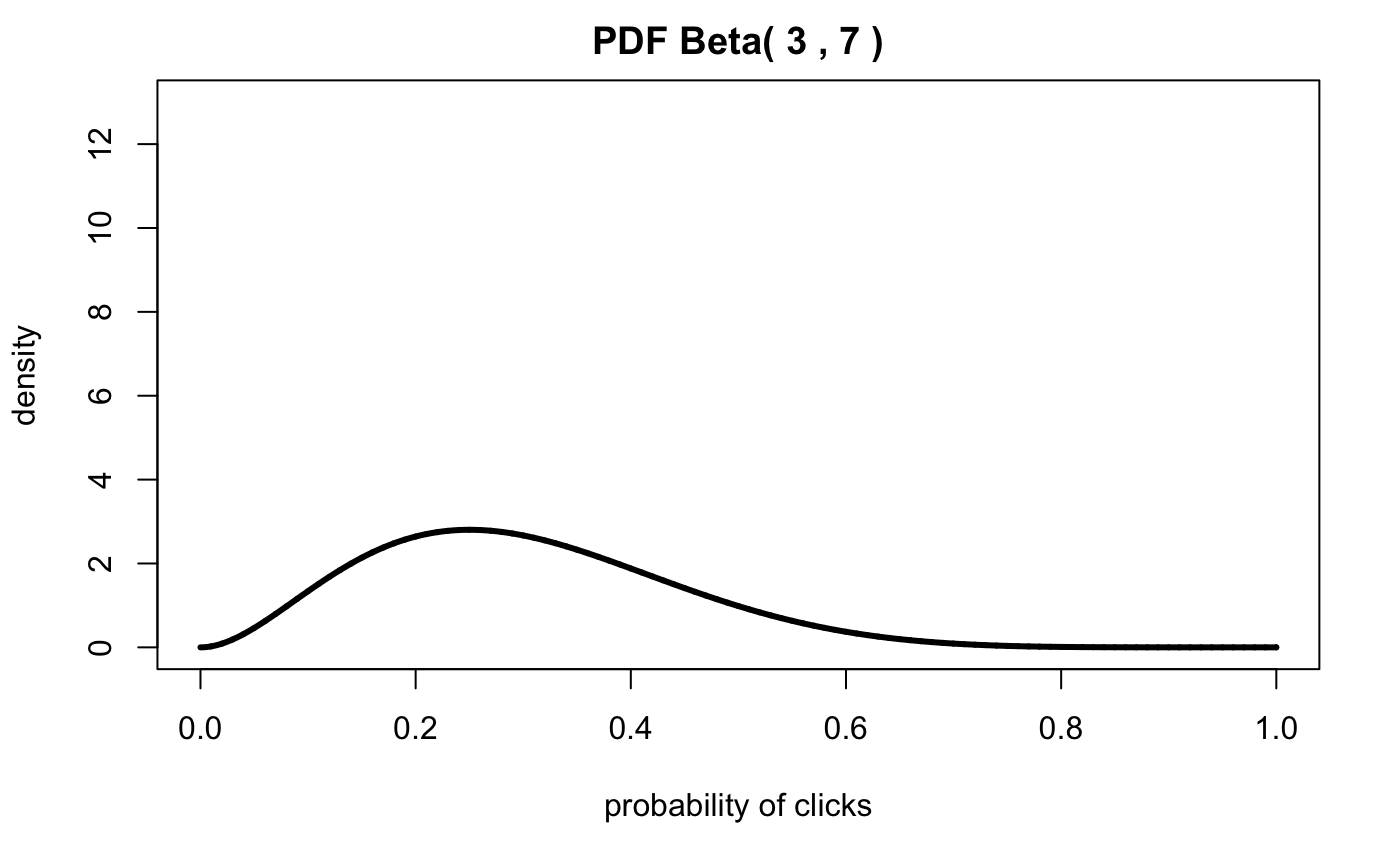
If we calculate the 95% confidence interval, it tells us that the click-through rate falls between 10% and 90%!
Now, let’s assume that previous email campaigns only yield a 2.4% success rate, let’s use Bayes Theorem to apply our prior probability to calculate the actual posterior probability we should expect to see.
Let’s assign a weak prior probability with \(\alpha = 1\) and \(\beta = 41\). I define “weak” as N events \(N < 45\).
alpha.1 <- 1
beta.1 <- 41
plotbeta(alpha.1,beta.1,xs.all,c(0,40))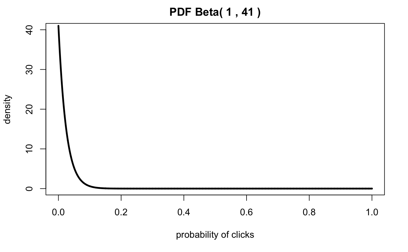
Combining the Prior Probability and the Likelihood Parameters to Yield the Posterior Probability
Specifically for the Beta distribution, we can easily combine parameters of the prior and the likelihood to yield the posterior probability:
\[Beta (\alpha_{prior} + \alpha_{likelihood}, \beta_{prior} + \beta_{likelihood})\]This is why I think anyone learning Bayes Statistics should start off with the Beta distribution because it’s easy to calculate the posterior probability.
After we understand the core essence of Bayesian Statistics, we can move on to more complicated models such as linear models and more generalized linear models.
Let’s graph the likelihood and the posterior probability now:
plot(xs.all, dbeta(xs.all,alpha + alpha.1, beta + beta.1),type='l',lwd=3,col='red',
     ylab='density',
     xlab='probability of clicks')

lines(xs.all,dbeta(xs.all, alpha, beta),col='black',lwd=3,lty=2)
legend(x='topright',
       legend=c('With Prior', 'No Prior'),
       col=c('red','black'),
       lty=c(1,1),
       ncol=1 )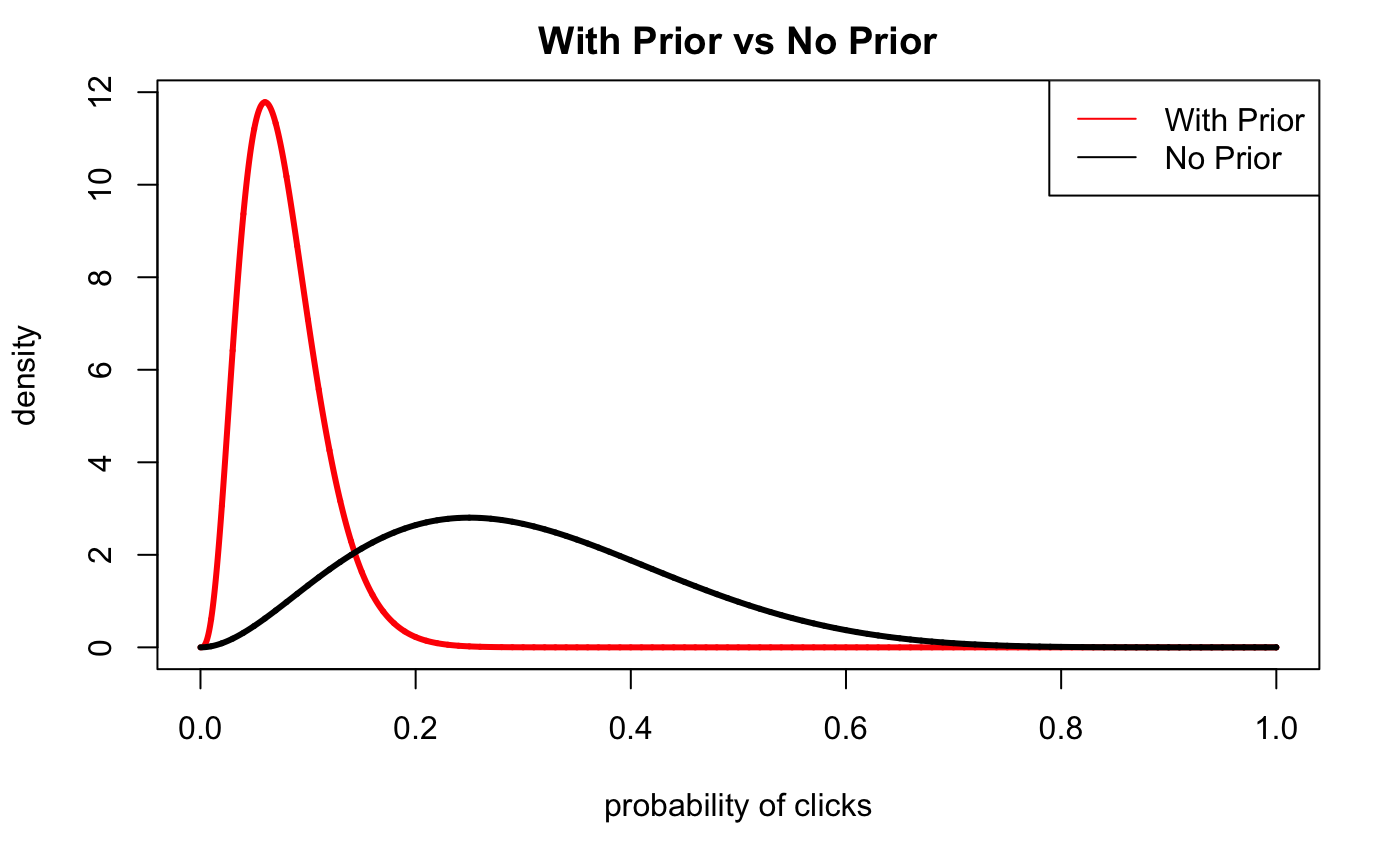
We can see that even with a weak prior, we have significantly shifted the distribution to a distribution that makes more intuitive sense given our past knowledge and experiences; we’ve reallocated credibility across the different possible probabilities from our likelihood.
Let’s go back and recalculate the posterior distribution with more data.
Assume that the day has progressed and we have more data from our email campaign. We have sent out 100 total emails with 25 people clicking through the email.
\(\alpha=25\)
\(\beta=75\)
alpha = 25
beta = 75
plot(xs.all, dbeta(xs.all,alpha + alpha.1, beta + beta.1),type='l',lwd=3,col='red',ylim=c(0,20),xlim=c(0,0.4),
     ylab='density',
     xlab='probability of clicks',
     main='With Prior vs No Prior')

lines(xs.all,dbeta(xs.all, alpha, beta),col='black',lwd=3,lty=2)
legend(x='topright',
       legend=c('With Prior', 'No Prior'),
       col=c('red','black'),
       lty=c(1,1),
       ncol=1 )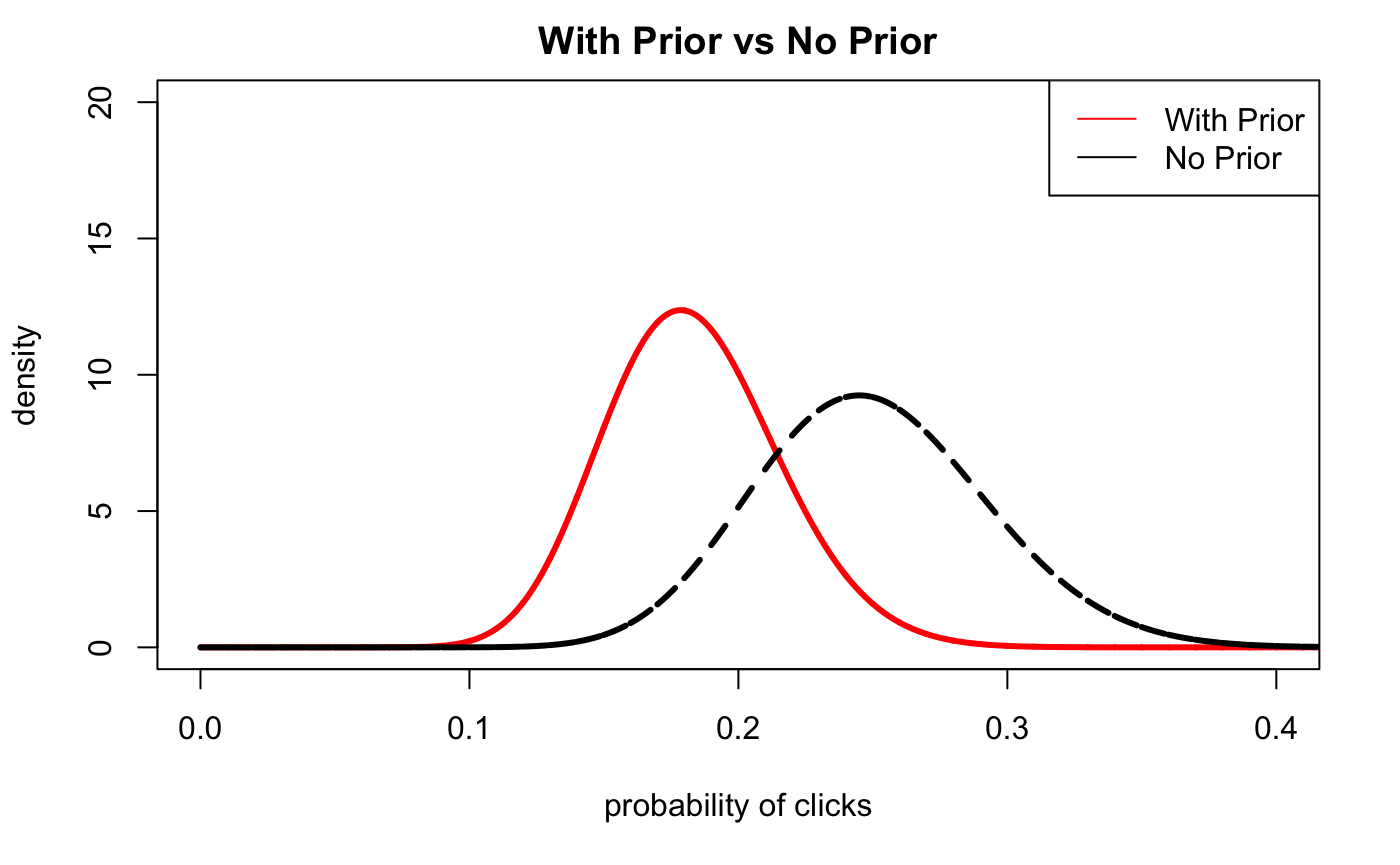
Assume we show these results to the Marketing Manager in charge of the email campaign beleves that our priors should be a lot stronger. Let’s update our posterior probability with a stronger prior:
\(\alpha_{prior} = 5\)
\(\beta_{prior} = 41\)
plot(xs.all, dbeta(xs.all,alpha + alpha.3, beta + beta.3),type='l',lwd=3,col='red',xlim=c(0,0.4),
     ylab='density',
     xlab='probability of clicks',
     main='With Prior vs No Prior')

lines(xs.all,dbeta(xs.all, alpha, beta),col='black',lwd=3,lty=2)
legend(x='topright',
       legend=c('With Prior', 'No Prior'),
       col=c('red','black'),
       lty=c(1,1),
       ncol=1 )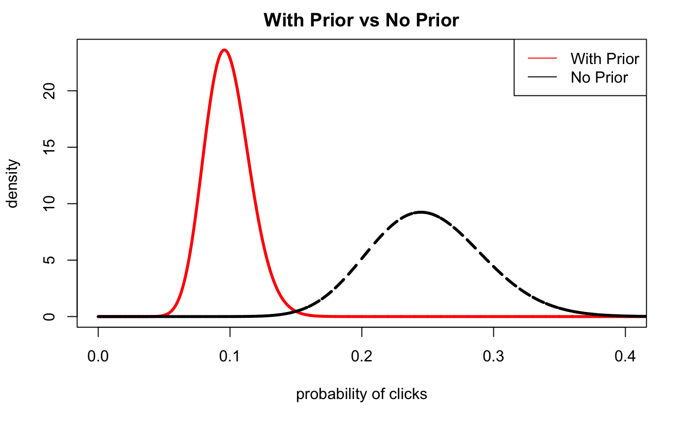
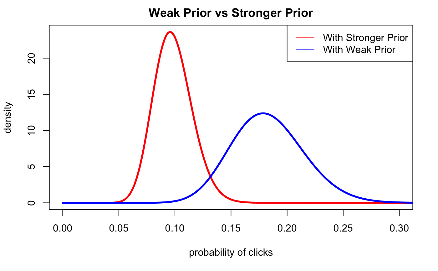
To make it clear, let’s graph the two different posterior probabilities by themselves to see how the strength of a prior probability can drastically move the likelihood.
plot(xs.all, dbeta(xs.all,alpha + alpha.3, beta + beta.3),type='l',lwd=3,col='red',xlim=c(0,0.3),
     ylab='density',
     xlab='probability of clicks',
     main='Weak Prior vs Stronger Prior')

lines(xs.all,dbeta(xs.all, alpha + alpha.1, beta + beta.1),col='blue',lwd=3,lty=1)
legend(x='topright',
       legend=c('With Stronger Prior', 'With Weak Prior'),
       col=c('red','blue'),
       lty=c(1,1),
       ncol=1 )
Summary
Using the Beta distribution, we’ve shown how we can step through the mechanical application of Bayes Theorem. Graphing the different distributions that make up the components of Bayes Theorem proves to be valuable in understanding the relationship that the Prior Probability has with the Likelihood.
Fortunately the Beta distribution allows us to simply combine our alpha and beta parameters of our prior and likelihood distributions to yield the posterior probabilities.
Any other distribution will involve more simulations and computation power to compute the distributions for the prior, likelihood, and evidence using a technique called the Markov-Chain Monte Carlo (MCMC) method which I plan to write about later.
Sneak Preview on A/B Testing
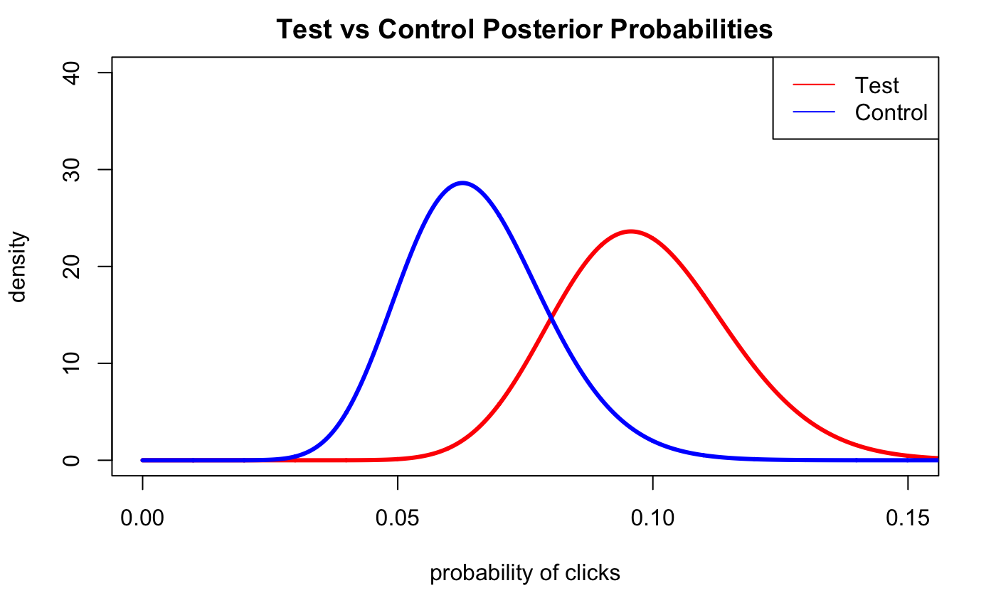
As a sneak preview on how we would use the posterior distributions to conduct an A/B test, imagine now we have split up our emails between Test and Control where we send a generic campaign message to our Control group and a more specialized message for the Test group.
We gather the data and graph the posterior probabilities of both the Test and Control:
alpha_control <- 15
beta_control <- 85

plot(xs.all, dbeta(xs.all,alpha + alpha.3, beta + beta.3),type='l',lwd=3,col='red',xlim=c(0,0.15),ylim=c(0,40),
     ylab='density',
     xlab='probability of clicks',
     main='Test vs Control Posterior Probabilities')

lines(xs.all,dbeta(xs.all, alpha_control + alpha.3, beta_control + beta.3),col='blue',lwd=3,lty=1)
legend(x='topright',
       legend=c('Test', 'Control'),
       col=c('red','blue'),
       lty=c(1,1),
       ncol=1 )
```